Based on Data Science Tutorial in Python of Ambica Nandimandalam
We can check the effectiveness of an algorithm by choosing an open dataset. At first, it’s really important to visualize your dataset in proper way. Visualization matters..
Let’s import relevant libraries for our analysis. Pandas is for analysis and modelling, Numpy and Matplotlib for scientific computing.. Scikit-Learn is a Python module for ML.
import pandas as pd
import numpy as np
import matplotlib.pyplot as plt
from sklearn.svm import SVC
from sklearn.metrics import accuracy_score
from sklearn.metrics import classification_report
from sklearn.metrics import confusion_matrix
%matplotlib inline
We could try a tested dataset. Iris is a flower dataset which contains 3 classes of 50 instances each, and each class refers to a type of iris plant. This type of data is appropriate for demonstration and/or educational purposes..
Iris = pd.read_csv("http://archive.ics.uci.edu/ml/machine-learning-databases/iris/bezdekIris.data",
names = ["Sepal Length", "Sepal Width", "Petal Length", "Petal Width", "Class"])
Take a look at the data.. Usually, datasets need a lot of work to prepare them for analysis. However, this is a structured dataset, meaning that we can get an idea by reading a few lines ..
print(Iris.head(10))
It’s easy to see the structure of this dataset - it includes four features and three classes..
   Sepal Length  Sepal Width  Petal Length  Petal Width        Class
0           5.1          3.5           1.4          0.2  Iris-setosa
1           4.9          3.0           1.4          0.2  Iris-setosa
2           4.7          3.2           1.3          0.2  Iris-setosa
3           4.6          3.1           1.5          0.2  Iris-setosa
4           5.0          3.6           1.4          0.2  Iris-setosa
5           5.4          3.9           1.7          0.4  Iris-setosa
6           4.6          3.4           1.4          0.3  Iris-setosa
7           5.0          3.4           1.5          0.2  Iris-setosa
8           4.4          2.9           1.4          0.2  Iris-setosa
9           4.9          3.1           1.5          0.1  Iris-setosa
Additionally, it’s common practice in data analysis to get information for basic statistics..
print(Iris.describe())
       Sepal Length  Sepal Width  Petal Length  Petal Width
count    150.000000   150.000000    150.000000   150.000000
mean       5.843333     3.057333      3.758000     1.199333
std        0.828066     0.435866      1.765298     0.762238
min        4.300000     2.000000      1.000000     0.100000
25%        5.100000     2.800000      1.600000     0.300000
50%        5.800000     3.000000      4.350000     1.300000
75%        6.400000     3.300000      5.100000     1.800000
max        7.900000     4.400000      6.900000     2.500000
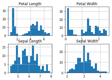
Histogram, it’s the first step to visualise basic statistical info about your data.. Try histograms with large and small number of bins and select the more informative ..
Iris.hist(bins=20)

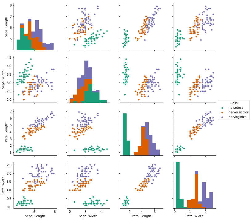
Pairplot could give you an advanced visual info about your data.. For example, which class is most seperable and which feature contributes the most ..
import seaborn as sns
sns.pairplot(Iris, hue = 'Class', palette = 'Dark2')

Now, it’s time to train and test an algorithm, but in order to do this effectively we need random data .. so, we can, technically, randomize our data ..
iris_array = Iris.values
np.random.shuffle(iris_array)
The next step would be to split the data.. We need two subdatasets - the first one for training and the second for testing. The point is the ‘right’ size for these subdatasets, a small training set would be a wrong guide to set up our algorithm, on the other side an extremely large training algorithm would be a waste of time. However, these questions are tricky when we deal with unstructured datasets.
X_train = iris_array[:80][:,0:4]
Y_train = iris_array[:80][:,4]
X_test = iris_array[-20:][:,0:4]
Y_test = iris_array[-20:][:,4]
Let’s train our model. We could use several models, however, a good choice for our data would be a Support Vector Machine.. SVM is a discriminative classifier meaning that, given a training dataset (supervised learning), the algorithm categorizes each new class.. defining the optimal mathematical region for each class..
svc = SVC()
svc.fit(X_train,Y_train)
This is our classifier..
SVC(C=1.0, cache_size=200, class_weight=None, coef0=0.0,
  decision_function_shape='ovr', degree=3, gamma='auto', kernel='rbf',
  max_iter=-1, probability=False, random_state=None, shrinking=True,
  tol=0.001, verbose=False)
Therefore, we are going to get predictions from our model ..
predictions = svc.predict(X_test)
print("Predicted Results:")
print(predictions)
Predicted Results:
['Iris-setosa' 'Iris-virginica' 'Iris-setosa' 'Iris-setosa' 'Iris-setosa'
 'Iris-setosa' 'Iris-virginica' 'Iris-virginica' 'Iris-virginica'
 'Iris-versicolor' 'Iris-virginica' 'Iris-virginica' 'Iris-versicolor'
 'Iris-virginica' 'Iris-virginica' 'Iris-versicolor' 'Iris-versicolor'
 'Iris-virginica' 'Iris-setosa' 'Iris-setosa']
And we will compare them with the Actual Results ..
print("Actual Results:")
print(Y_test)
Actual Results:
['Iris-setosa' 'Iris-versicolor' 'Iris-setosa' 'Iris-setosa' 'Iris-setosa'
 'Iris-setosa' 'Iris-virginica' 'Iris-virginica' 'Iris-virginica'
 'Iris-versicolor' 'Iris-virginica' 'Iris-virginica' 'Iris-versicolor'
 'Iris-virginica' 'Iris-virginica' 'Iris-versicolor' 'Iris-versicolor'
 'Iris-virginica' 'Iris-setosa' 'Iris-setosa']
So, the Accuracy Rate will be pretty high - meaning that our classifier has done a good job for this type of data ..
print("Accuracy rate: %f" % (accuracy_score(Y_test, predictions)))
Accuracy rate: 0.950000
Also, with a Confusion Matrix, we will have a more complete picture for our model at this particular dataset. However, SVC model belongs to Supervised Learning, meaning that its effectiveness will be limited for datasets with completely different structure ..
print(confusion_matrix(Y_test, predictions))
[[7 0 0]
 [0 4 1]
 [0 0 8]]
print(classification_report(Y_test, predictions))
At last, we check the Classification Report.. Precision is a ratio that shows the Accuracy with FP, while recall is the respective ratio with FN. Therefore, we conclude that our model with Setosa and Versicolor classes works pretty well, however, it may need some corrective actions for Virginica because it presents too many FP..
                 precision    recall  f1-score   support

    Iris-setosa       1.00      1.00      1.00         7
Iris-versicolor       1.00      0.80      0.89         5
 Iris-virginica       0.89      1.00      0.94         8

    avg / total       0.96      0.95      0.95        20